Image reconstruction from CT scans

by Stoica-Marcu Floris-Andrei
Ovidius University of Constanta

CT machines work by shooting out thin X-Rays that pass through the material to a detector plate.

By shooting many rays in different angle configurations for a single horizontal slice of the material, the CT machine and reconstruction algorithm is able to reconstruct the slice.

Combining multiple horizontal slices vertically results in a 3D reconstruction of the scanned material.

For demonstration purposes, this application uses brain imaging data from the OpenNeuro Dataset ds000102.

Resolution

The machine is fine-tuned, based on parameters such as number of rays, angles and detector performance, for a certain resolution - i.e. number of voxels able to reconstruct.

In our 2D example, this is represented by a cell size of 5x5px, downsampled and calculated from an image of 256x256px.

X-Ray mechanism - analytic

Each X-ray beam passing through the material is attenuated by the linear attenuation coefficient \( \mu \) along its path.

According to Lambert-Beer's law, the intensity at the exit point B, starting from intensity \( I_A \) at point A, is:

$$ I_B = I_A \, e^{-\int_A^B \mu(s) \, ds} $$

The total attenuation \( \beta \) along the path is:

$$ \beta = \int_A^B \mu(s) \, ds = -\ln(I_B / I_A) $$

In discrete space, each voxel the ray passes through contributes to the total attenuation, exponentially reducing the beam's intensity.
Preparing our scan

Faking a CT machine

If you assume that a CT machine is expensive ... You would be correct! Thus, we will need to fake its results so that we may reconstruct the fake results!

Trust me, this will make a lot more sense later.

The plan is to stick any 2D grayscale image into our virtual scanner and see how our reconstruction algorithm performs.

I chose a fan-beam circular layout for our virtual CT machine. It was a fun thing to code and it should also look quite familiar to you.

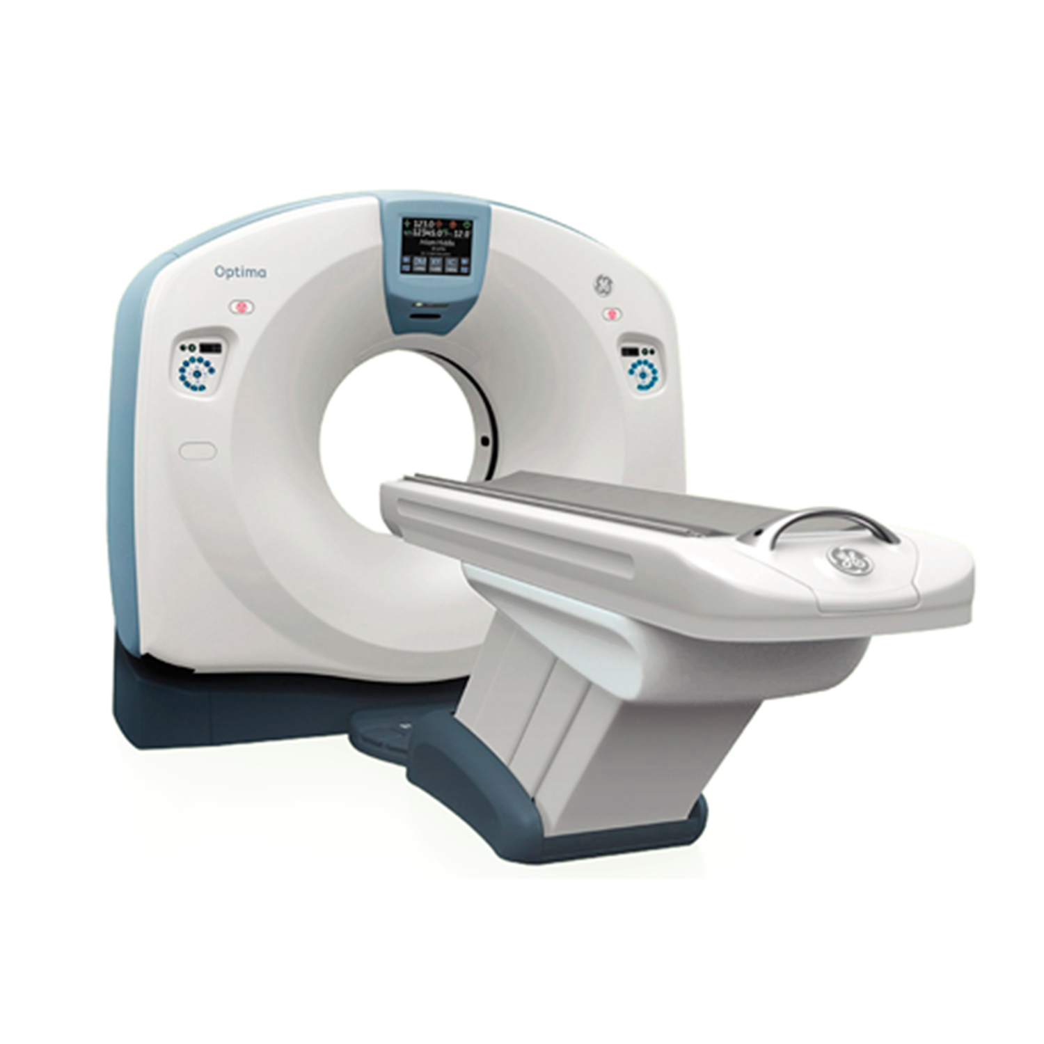
CT scanner that we are trying to fake

Discretization

How We Compute the Line Integral

To compute the projection value for each ray, we need to calculate the line integral \( \beta = \int_A^B \mu(s) \, ds \), which represents the total attenuation along the ray path.

Because the image is divided into a grid of voxels, we calculate the line integral by first determining which voxels it intersects and compute the length of the ray segment within each voxel.

The total attenuation for a ray is then:

$$ \beta = \sum_{i,j} \mu_{i,j} \cdot l_{i,j} $$

where \( l_{i,j} \) is the length of the ray segment inside voxel (i,j).

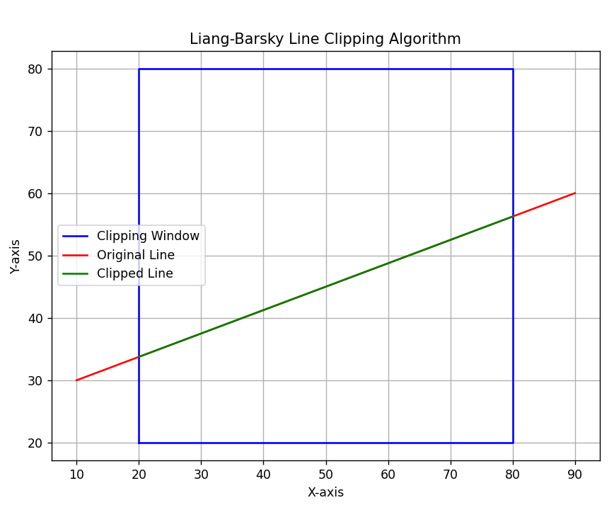
To compute \( l_{i,j} \), we use the Liang-Barsky line clipping algorithm. This function efficiently computes the intersection of a ray with a rectangular voxel, returning the entry and exit points and the segment length.

The algorithm works by parameterizing the ray as \( P(t) = (ox, oy) + t \cdot (dx, dy) \), t ≥ 0, and finding the valid t range [t1, t2] where the ray is inside the rectangle. The length is then (t2 - t1) * ||(dx, dy)||.

Liang-Barsky line clipping algorithm illustration

By iterating over all voxels that could potentially intersect the ray (determined by bounding box checks), we accumulate the contributions to get the final projection value.

Discretization of the rays

To apply the reconstruction algorithm, we need to discretize the problem. The continuous image is divided into a grid of square voxels, each with an attenuation coefficient μ. In our example, we use a 50x50 grid, representing the resolution of our virtual CT scanner. The black/white values of the pixels represent a lower or higher attenuation.

Each ray is discretized into a set of measurements by computing the line integral of the attenuation along the ray path - also known as the projection value \( \beta \) .

The Radon transform is a mathematical operation that computes the integrals of a function along all possible lines, forming the basis of tomographic imaging. In CT reconstruction, it transforms the original image into its projection data, which we then invert to recover the image.

This discretization transforms the continuous Radon transform into a discrete system of linear equations: A x = b, where A is the system matrix containing the intersection lengths of each ray with each voxel, x is the vector of voxel intensities, and b is the vector of measured projections.

Kaczmarz Reconstruction Algorithm

The Kaczmarz Method

The Kaczmarz algorithm is an iterative method for solving overdetermined systems of linear equations. It works by projecting the current estimate onto the hyperplanes defined by each equation in sequence.

For each equation i: \( \langle a_i, x \rangle = b_i \), the update is:

$$ x^{k+1} = x^k + \frac{b_i - \langle a_i, x^k \rangle}{\|a_i\|^2} a_i $$

where \( a_i \) is the i-th row of the system matrix A, \( b_i \) is the i-th measured projection, and \( \|a_i\|^2 \) is the squared Euclidean norm of the row vector \( a_i \).

In CT reconstruction, each ray corresponds to an equation \( \langle a_i, x \rangle = b_i \), where \( b_i \) is the measured line integral \( \beta \) and \( a_i \) contains the intersection lengths \( l_{i,j} \) with voxels. The Kaczmarz algorithm cycles through rays, updating \( x \) as \( x^{k+1} = x^k + \frac{b_i - \langle a_i, x^k \rangle}{\|a_i\|^2} a_i \), adjusting voxel intensities to match each ray's measurement.

The algorithm converges to a solution that minimizes the least squares error. In practice, we stop after a fixed number of iterations or when the residual falls below a threshold.

This method is particularly suitable for large systems and can handle noisy data effectively.

Technical Details

Implementation in C with Raylib

The project is written in C for efficient memory control and performance in computational tasks like image reconstruction. Raylib, a lightweight game development library, handles graphics, windowing, and user input, allowing focus on the core Kaczmarz algorithm.

Web Deployment with WebAssembly

C code is compiled to WebAssembly (WASM) using Emscripten, enabling high-performance browser execution. This provides an interactive demo without downloads, with JS bindings for stage control and resource preloading.

References

"Liang-Barsky Algorithm." Wikipedia. Wikimedia Foundation. https://en.wikipedia.org/wiki/Liang%E2%80%93Barsky_algorithm. Accessed 18 Dec. 2025.

"Liang-Barsky Algorithm." GeeksforGeeks. https://www.geeksforgeeks.org/computer-graphics/liang-barsky-algorithm/. Accessed 18 Dec. 2025.

"Kaczmarz method." Wikipedia. Wikimedia Foundation. https://en.wikipedia.org/wiki/Kaczmarz_method. Accessed 18 Dec. 2025.

Radon, Johann. "On the determination of functions from their integral values along certain manifolds." IEEE Transactions on Medical Imaging 5 (1986): 170-176.

Kelly, A.M., Uddin, L.Q., Biswal, B.B., Castellanos, F.X., Milham, M.P. (2008). Competition between functional brain networks mediates behavioral variability. Neuroimage, 39(1):527-37.

Mennes, M., Kelly, C., Zuo, X.N., Di Martino, A., Biswal, B.B., Castellanos, F.X., Milham, M.P. (2010). Inter-individual differences in resting-state functional connectivity predict task-induced BOLD activity. Neuroimage, 50(4):1690-701. doi: 10.1016/j.neuroimage.2010.01.002. Epub 2010 Jan 15. Erratum in: Neuroimage. 2011 Mar 1;55(1):434.

Mennes, M., Zuo, X.N., Kelly, C., Di Martino, A., Zang, Y.F., Biswal, B., Castellanos, F.X., Milham, M.P. (2011). Linking inter-individual differences in neural activation and behavior to intrinsic brain dynamics. Neuroimage, 54(4):2950-9. doi: 10.1016/j.neuroimage.2010.10.046.

OpenNeuro Dataset ds000102. https://github.com/OpenNeuroDatasets/ds000102. Accessed 18 Dec. 2025.

Special Thanks

Special thanks to Dean Aurelian Nicola, who taught the CT reconstruction class and whose challenging and engaging lectures made it the most memorable part of my master's degree programme.

Equally, thanks to Prof. Dr. Dorin-Mircea Popovici, whose infectious enthusiasm and remarkable work in the CERVA lab continuously inspire me.

Loading...